1.2 Basis function regression

1.2 Basis function regression

We can illustrate the training of a model in a simple case where $x_n$ and $y_n$ are two real numbers, the loss is the mean squared error: \(\mathscr{L}(w)=\frac{1}{N}\sum_{n=1}^N(y_n-f(x_n;w))^2 \tag{1.1}\)

and $f(\cdot;w)$ is a linear combination of a predefined basis of functions $f_1,…,f_K$, з $w=(w_1,…,w_K)$: \(f(x;w)=\sum_{k=1}^Kw_kf_k(x)\)

Since $f(x_n;w)$ is linear with respect to the wks and $w_k$ and $\mathscr{L}(w)$ is quadratic with respect to $f(x_n;w)$, the loss $\mathscr{L}(w)$ is quadratic with respect to the $w_k$s, and finding $w^*$, that minimizes it boils down to solving a linear system. See Figure 1.1 for an example with Gaussian kernels as $f_k$.

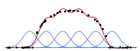
Figure 1.1: Given a basis of functions (blue curves) and a training set (black dots), we can compute an optimal linear combination of the former (red curve) to approximate the latter for the mean squared error.